Self-Checking Assessments in Google Sheets with Conditional Formatting
There are several tools that can be used for this sort of self-assessment. One great option is to use Google Sheets with conditional formatting.
There are so many excellent tools for online assessment including Google Forms, Quizlet, Kahoot, Flippity, Quizizz, and more. In addition to providing teachers with data on student performance, online quizzes can also be valuable simply for student self-assessment.
With self-assessments the purpose is for the student to test themselves, see if they are correct or not, and usually retry until they get the right answer. Grades are not collected, because by the end the student should have every question correct. The point is to let the learner practice, see what they do and do not understand, and then work toward improvement.
There are several tools that can be used for this sort of self-assessment. One great option is to use Google Sheets with conditional formatting. This allows you to provide feedback based on what the student types in for their answers, so they can identify and work on questions they are struggling with.
To help make this easier, I have created a "Self-Checking Assessment Template" for Google Sheets. See below for a link to get your own copy, along with directions on how to use it, and some behind-the-scenes explanations of how it works.
Self-Checking Examples
Before we check out the templates, it may be best to start with some completed examples to show the final product. For my examples I used some Ohio trivia (since that is where I live). Click on either link below to get your own copy of a self-checking example:
Ohio Trivia (without hints) - Google Sheets link
Tech & Learning Newsletter
Tools and ideas to transform education. Sign up below.
Ohio Trivia (with hints) - Google Sheets link
Once you get your copy of the Ohio Trivia example, you can begin typing in your answers in the "Answers" column. If you get an answer correct, the cell will fill in with green (because of conditional formatting).
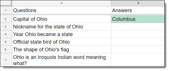
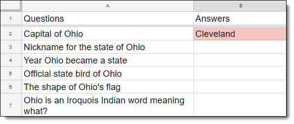
If you type in the incorrect answer, then the cell will turn red. You can then try again until you get the correct answer.
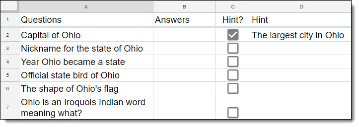
For the example that includes the "Hints" option, you can check the box to get a hint displayed if needed.
Self-Checking Templates
To make your own self-checking assessments, you can click the links below to get a copy of either template:
Self-Checking Template (without hints) - Google Sheets link
Self-Checking Template (with hints) - Google Sheets link

Directions for Use
Once you have a copy of the template, here is how you fill it out and set it up for use:
The template will have two tabs at the bottom, one titled "Questions" and one titled "Key".
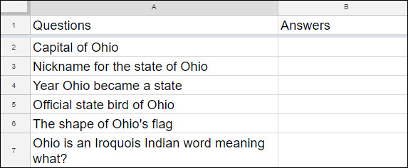
Type in your questions on the "Questions" tab, one question per row.
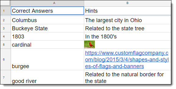
Next type in the answers on this "Key" tab, one per row, matching the rows on the "Questions" tab.
If you are using the templates that include the "Hints" option, then type in the hints on the "Key" tab, one per row, matching the rows on the "Questions" tab. Hints can include text, links, images and more.
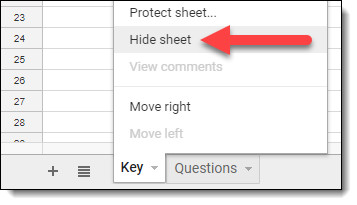
When all done, you can now share your Sheet with others.
*You can share the Sheet as view-only, and then users can make their own copy to fill out.
*Or you could use a tool like Google Classroom to make a copy of the Sheet for each student.
Conditional Formatting
For those interested in how the template actually works, the main feature of Sheets being used is conditional formatting. This is a setting in Sheets that allows you to format cells based on the content that is typed into the cells. In the past, this is how I created my "20-Color Pixel Art Template" and my "Long Multiplication template".
Here are the basic for how conditional formatting works:
- First, select the cell (or cells) you wish to apply the conditional formatting to.
- Next click "Format" in the top menu bar.
- Choose "Conditional formatting" from the drop-down menu.
- This will open a panel on the left titled "Conditional format rules".
- For "Apply to range" you can change which cells are affected if needed.
- For "Format cells if" you can choose the condition that needs to be met. This can include many options such as comparing text, numerical values, and dates, as well as more advanced custom formulas.
- For "Formatting style" you can choose how to format the cells if the above condition is met. This can include cell color, text color, bold, strike-through, and more.
- If you need to add more rules, you can click "Add another rule" and repeat the process.
- When all done, click "Done".
Now anytime someone types content into the cells, the conditional formatting rules will be checked. If the content that is typed in matches one of the rules, then the corresponding formatting will be applied to that cell.
For the Self-Checking Templates in this blog post, I used custom formulas in conditional formatting to take what the user types in on the "Questions" tab and compare that to the correct answers on the "Key"tab. If they match, the conditional formatting colors the cells in green, and if they do not match then the rule colors the cell red.
cross posted at www.controlaltachieve.com
Eric Curts is an education trainer and consultant with over 20 years' experience throughout the U.S. He is an authorized Google Education Trainer and a Google Certified Innovator. Read his blog at www.controlaltachieve.com and follow him on Google+ and @ericcurts on Twitter.
